A Superior Description of AC Behavior in Polycrystalline Solid Electrolytes with Current-Constriction Effects

Article information

Abstract

1. Introduction

The AC characterization technique is an indispensable tool for electroceramic materials, both conducting and dielectric, and for the devices comprising them. Although the technique is widely applied and is becoming more popular, the information derived there from is so far very limited and often disputable. The technique is far from being properly utilized. Mono-frequency capacitance analyses of the temperature- or bias-dependence of electroceramics and semiconductor devices suffer seriously from intrinsic frequency dispersions as well as from the overlapping of other responses. Universally observed frequency dispersions have been studied mostly using the AC conductivity or admittance spectra. Circuit analyses have been widely practiced on the other hand. Constant phase elements (CPEs) of impedance Z^*= 1/[Q(jω)^a], often represented as Q elements, may be considered as ‘magic’ elements. Employed as ‘generalized’ capacitors or resistors, they appear to allow plausible description of most real data. However, they are also the cause of much trouble in AC characterization. CPEs cannot unequivocally provide resistance or capacitance parameters, which can be related to the physical quantities sought for in AC characterization.

Although CPEs were originally introduced as ‘generalized’ resistors to describe the non-Debye responses of real dielectrics,1) presently they serve as ‘generalized’ capacitors in most AC characterization, in which the resistance effects are of primary interest for the evaluation of the conductivities and/or power dissipation in general. As noted previously,2) capacitance effects, which are less affected by local inhomogeneity and short-circuiting, may provide more reliable physical insights than can be obtained from resistance effects. In fact, as clearly shown in the beta alumina system,3) the strongly dispersive responses of solid electrolytes indicate the rather well-defined capacitance and frequency dispersion. Without any spectral evaluation, AC conductivity Arrhenius plots can directly reveal the current-constriction character of blocking effects in the polycrystalline beta alumina system. Parallel networks of the complex dielectric functions with the parameters directly indicated in the raw data can describe the AC responses over a wide temperature and frequency range. The parameters involved are only around ten in number. The analysis has been successfully applied to AgI4) and scandium NASICON analog.5)

The description of the dispersive AC behavior of the polycrystalline solid electrolytes with current constriction effects is now getting established.3–5) The present work intends to generally illustrate the new methodology using theoretical simulations. This work also demonstrates the problems in conventional bricklayer analysis for the dispersive response of many solid electrolyte systems. Brick-layer analysis has been applied to solid electrolytes with blocking grain boundaries. Brick-layer modelling of polycrystalline electroceramics formally integrates well with the space charge mechanism for blocking effects. The grain boundary resistance and capacitance can be parameterized in terms of the charge depletion layers along the grain boundaries, as is well-known for semiconductor systems. Although large carrier concentration in ionic conductors causes difficulty in the quantitative estimation of the grain boundary parameters, the space charge theory can explain the higher activation energy necessary for transport across grain boundaries than is the case for the transport in the bulk. In the case of current-constriction grain boundary effects showing similar activation energy as for the bulk transport, grain boundary parameters from brick-layer analysis cannot be clearly explained even in theoretical simulations.6,7) It can be concluded that conventional brick-layer analysis has problems both in theory and in practice for the description of dispersive responses of polycrystalline solid electrolytes with current-constriction effects.

2. Methods

Impedance simulations as a function of temperature and frequency were performed with Matlab (Mathworks, USA). Individual spectra were also simulated by Zview (Scribner Ass. Inc., USA). Parametric analysis of the impedance spectra by complex non-linear least squares fitting was also performed with Zview. The numerical Kramers-Kronig test was performed using the KK-test program provided by Prof. B. Boukamp.8,9)

3. New Capacitance-centered Spectroscopy

The new approach essentially follows textbook dielectric spectroscopy in which the polarization contributions such as space charge at grain boundaries (ɛ_GB) (and electrodes) as well as the relaxation mechanism in the bulk (ɛ_C) are additive to the static dielectric constant (ɛ_S), as schematically illustrated in Fig. 1. Two polarization processes are described by RC series circuits or Debye responses in solid lines. Non-Debye responses observed in real dielectric systems are formulated as Cole-Cole, Cole-Davidson or, in general, Havriliak-Negami functions1,10,11)

Fig. 1

Variation of the dielectric constants with frequency for a polycrystalline ceramic ionic conductor with Debye polarizations in the bulk (ɛ_C) and from the grain boundaries (ɛ_GB). Dashed lines represent Havriliak-Negami-type relaxations.

No circuit analogs are present except for the Debye case with β=γ=1. The low-frequency-limiting frequency power-law exponent or log-log slope is β, and the high-frequency limiting slope is −βγ. The peak frequency of a Havriliak-Negami response is12,13)

When γ ≠ 1, the peak frequency is shifted from τ⁻¹ for β = γ = 1 (Debye) and β < 1 (γ = 1) (Cole-Cole). The peak frequency becomes higher when γ < 1 for the negatively skewed dielectric spectra and lower when γ > 1 for the positively skewed spectra. It should be noted that under the condition of β·γ ≤ 1, a well-behaved complex dielectric function with positive skewness is allowed for β > 1.14)

In Fig. 1, dashed-line Havriliak-Negami-type responses are compared with solid-line Debye relaxations. A Cole-Davidson type relaxation with β = 1 and γ ≈ 0.4 and dielectric strength ɛ_C in the bulk solid electrolytes approximately represents the apparent dielectric effects due to the mobile charge carriers.3–5) This type of Cole-Davidson approximation was suggested for the exact Laplace-Fourier transform of the stretched exponential temporal response, exp(−t^β_k) with β_K = 1/3.15–21) Together with the true dielectric capacitance C₀, it is named the CK1 model. Mobile charge carrier origin is shown in the temperature dependence of the relaxation time constants τ_HN as τ⁻¹T ∝ exp(−E_σ/k_BT).

The dielectric spectrum in Fig. 1 suggests that the three-dimensional polarization effects in the polycrystalline microstructure are similarly described as the polarization process in the bulk. Unlike the CK1 type response, which is due to the mobile charge carriers with well-defined frequency dispersion as β_K = 1/3 or γ ≈ 0.4, the dispersion character of the current constriction effects should vary from sample to sample. These constants are, however, determined by the microstructure and thus independent of the temperature as long as the conduction mechanism does not change. An example with β = 0.6 and γ = 0.7 is shown schematically in Fig. 1. For a beta alumina sample, a Cole-Davidson type equation with β = 1 and γ = 0.23 was found.3) On the other hand, for the scandium NASICON analog,5) an oppositely (positively) skewed function was employed with β = 0.59 and γ = 1.67 or βγ ≈ 1.

Such additive capacitance effects are connected in parallel in the circuit analogy. The equivalent circuits thereof are shown in Fig. 2(a, b). Two polarizations are represented by the ideal RC Debye circuits (a) and by the Havriliak-Negami function indicated by ‘H’ (b), respectively. Geometric capacitance from the dielectric constant ɛ_S is represented by the ideal capacitor C₀. Finite dielectric loss can be represented by a CPE with a value of a slightly less than 1.

Fig. 2

Equivalent circuits for the spectra in Figs. 3 and 4. ‘H’ represents a Havriliak-Negami dielectric response with power law exponents β and γ. The parameters for (a) and (b) are shown in Table 1. The fit results for the circuit (c) are shown in Table 2.

The models include an ideal Warburg response or CPE with a=0.5 in series connection to the sample resistance R_T. In the recent work on beta alumina3) and AgI,4) the electrode response of solid electrolytes with quasi-reversible electrodes is shown to be a surprisingly ideal Warburg type with the temperature dependence closely related to the bulk conduction as E_σ/2. The relation may be explained by the RC transmission line expression of the Warburg impedance which is ZW*=R/jωC, where the resistance represents the bulk conduction process in solid electrolytes.

Parameters of a realistic solid electrolyte system are presented in Table 1. As all the parameters are either constant or have a well-defined temperature dependence represented by E_σ, only 12 parameters are needed to simulate the temperature as well as the frequency dependence, as shown in Fig. 3. It should be noted that the exponent γ ≈ 0.4 for the approximate CK1 behavior is a constant fixed by a physical mechanism. With these parameters, AC behavior can be simulated over a wide temperature (1 ≤ 1000/T ≤ 6) and the frequency range (−2 ≤ Log(f/Hz) ≤ 6). The Bode plots in (a)–(f) are drawn every 0.2 in 1000/T and AC conductivity curves in (g, h, i) are for every 0.5 in Log(f/Hz).

Table 1

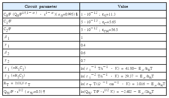
Parameters of the Equivalent Circuit of Fig. 2(a,b) for the AC Simulations in Fig. 3. E_σ=0.5 eV; Shape Factor A/t=1 cm

Fig. 3

Capacitance (a,b,c) and admittance Bode plots (d,e,f) and AC conductivity Arrhenius curves (g,h,i) using the fit parameters of the equivalent circuit (Fig. 2) listed in Table 1. Left column graphs (a,d,g) are for the ideal Debye circuit with all the frequency exponents 1; right column graphs (c,f,i) include the finite dielectric loss in Q₀ as tanδ with δ = (1−a₀)π/2. The Bode plots (a–f) are for temperatures 1 to 6 in 1000/T at an interval of 0.2 from the top. The thick lines are for the temperatures 1, 2, 3, 4, 5, and 6 in 1000/T. The Arrhenius plots (g,h,i) are for frequencies 6 to −2 in Log(f/Hz) at an interval of 0.5.

In the hypothetical ideal Debye relaxations with the capacitance magnitudes C₁ and C₂, represented in Fig. 3(a,d,g), R₁ and R₂ elements corresponding to τ₁ and τ₂ are indicated. The AC behavior with ideal Debye-type relaxations is characterized by the admittance plateaus (d) and the Arrhenius slopes (g) corresponding to the circuits (R₁R₂R_T) (in parallel), (R₂R_T), and R_T, all with the activation energy E_σ. The temperature dependence of the Warburg response is indicated by high-temperature low frequency traces with E_σ/2.

Characteristic bulk dispersion due to the mobile charge carriers represented by H₁ with β₁ = 1 and γ≈0.4 is indicated by the admittance Bode plots of the slope (1 − γ₁) (Fig. 3(e)). Admittance or conductivity Bode plots have been employed to present universally observed frequency dispersions.22–24 Many ionic conductors, crystalline and non-crystalline, show the relation (1 − γ₁) ≈ 0.60 ~ 0.67.25–28) The corresponding dispersion in the capacitance Bode plots of ω^γ₁−1 is not to be seen in the presence of the additional geometry capacitance contribution. Dispersion due to the current constriction, described by the H₂ component, is indicated by the exponent (1 − β₂γ₂). The respective dispersive responses are indicated in AC conductivity curves by the slopes γ₁E_σ and β₂γ₂E_σ (Fig. 3(h)). It should be noted that the Arrhenius slopes in Fig. 3(g) for the networks of R₁R₂R_T, R₂R_T, and R_T still serve as the boundary lines for different dispersion behavior. Exact positioning of the Arrhenius slope is possible for R_T, which is the only resistance parameter in circuit (b).

Finite dielectric loss, characterized by the factor tanδ, leads to the so-called ‘nearly constant loss (NCL)’ behavior characterized by slope 1 in the admittance Bode plots (Fig. 3(f))3,4,15,29–35) and in the flat AC conductivity curves proportional to ω (Fig. 3(i)), because Y′ = ωC′ tanδ ≈ ωC₀ tanδ. It should be noted that the frequency independent loss factor can be described by a CPE or Q with a ≈ 1 as δ = (1 − a)(π/2). Superlinear behavior with slope 2, universally observed at frequencies as high as GHz and THz,36) can be attributed to the small residual series resistance.3,4) A stray resistance of a few kΩ in parallel to the inductance from the setup leads to the superlinear behavior for the experimental EIS frequency range below 10 MHz.4) The present equivalent circuit approach can thus comprehensively describe different types of the universal dispersive responses. Simulations as shown in Fig. 3 with parameters around 10 in number excellently match the experimental data for beta alumina,3) AgI,4) and the scandium NASICON analog.5) The new approach is applicable to many other solid electrolyte systems; analysis for such systems will appear in following publications.

According to the CK1 model, the dielectric strength due to mobile charge carriers has a slight temperature dependence as5,19)

where N is the maximum mobile charge density and λ is the fraction of the charge q that is mobile and d is the rms single hop distance for the hopping entity. Decrease by the factor 2 would occur for the temperature increase from 500 K to 1000 K. Experimentally, C₂ as well as C₁ slightly decreases with temperature, supporting the idea of the common origin of the mobile charge carriers. The T⁻¹ dependence in C₁ and C₂ is neglected in the present simulations.

4. Problems of Brick-layer Analysis

Figure 4 displays the complex plane presentation in impedance of the spectra at 1000/T=1 (a), 2 (b), 3 (c), 4 (d), and 5 (e). Their Bode plots are indicated in thicker lines in Fig. 3. Debye responses (left), dispersive responses in Havriliak-Negami equations with β₁ = 1, γ₁ = 0.4, β₂ = 0.6, γ₂= 0.7 (middle), and with the dielectric loss factor tanδ, δ = (1 − a₀)(π/2) (a₀ = 0.995) in addition (right) are shown. The numbers represent the logarithmic frequencies. The frequency range, distinguished in the impedance plane presentation, is shown to be quite limited because the impedance becomes vanishingly small at high frequencies. The respective spectra can be also simulated by Zview program using model DE-28 for the Havriliak-Negami dielectric function.

Fig. 4

Impedance spectra at 1000/T=1 (a), 2 (b), 3 (c), 4 (d), and 5 (e) for the Debye responses (left), for the dispersive responses in the Havriliak-Negami equations with β₁=1, γ₁=0.4, β₂=0.6, γ₂=0.7 (middle), and with the additional dielectric loss factor tanδ, δ = (1 − a₀)(π/2) (a₀ = 0.995) (right).

Complex plane trajectories obtained from the parameters in Table 1 should be of the same shape at all temperatures when simulated for any arbitrarily wide frequency range. Only the magnitude changes according to the activation energy E_σ. The solid-line spectra (a) to (e) indicate the spectra at different temperatures; these spectra would be experimentally limited in the frequency range, e.g. −2 to 6 in Log(f/Hz). (The measurements can be also limited in terms of the maximum impedance magnitude allowed for the specific impedance analyzers.) Results for measurements at 1000/T = 2 and 3, shown in Fig. 4(b) and (c), display more or less completely the visible features in the impedance plane, with the slope-one line response of the Warburg impedance extending indefinitely at lowering frequencies.

At this point, it may be good to recall the basics of non-linear least squares fitting for impedance analysis. Parametric analysis in impedance spectroscopy is performed using complex nonlinear least squares fitting, which minimizes, e.g.

In non-linear curve fitting, the difference between the measured and fitted values to be summed in the squares should be normalized by the respective standard deviation. Assuming similar relative errors in the nonlinear data, the normalization uses the measured data values or the fitted (theoretical) values. Compared to normal nonlinear least squares fitting, complex variable fitting procedures have further variations in the weighting methods.17,21) The normalization can be done by the respective real and imaginary values or, as in Eq. (4), by the magnitude of the complex variables. It has been shown previously37) that impedance data that cut the real axis at high frequency due to the inductance can be better described by normalization using impedance magnitude than using respective real and imaginary values. Complex non-linear least squares fit results for the data in Fig. 4, using the brick-layer model in Fig. 2(c), which minimizes the sum of the squares according to Eq. 4 (which is the default weighting method in Zview program), are presented in Table 2 and Fig. 5.

Table 2

The Fit Results of the Impedance Spectra in Fig. 4 according to the Conventional Brick-layer Model Shown in Fig. 2(c)

Fig. 5

Complex non-linear least squares fit results for the data in Fig. 4, obtained using the brick-layer model in Fig. 2(c), which minimize the sum of the squares according to Eq. (4). The numerical values are given in Table 2.

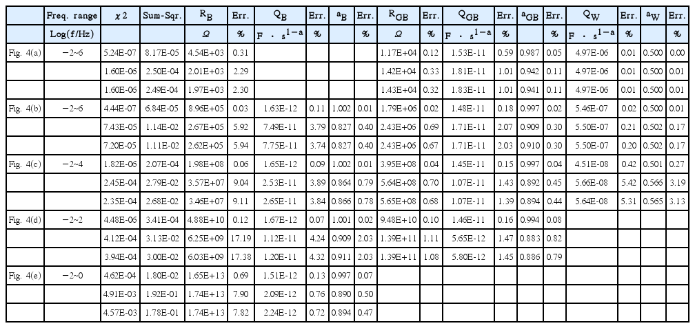
The spectrum at 1000/T=1 in Fig. 4(a) illustrates a typical high-temperature situation in which the high frequency arc cannot be measured due to limitations in the experimental frequency range. For such measurements, the component Q_B cannot be considered in the modeling. For the spectra simulated by the Debye relaxations on the left, compared to R_B/R_GB= 0.507 from the exact two arc analysis discussed in the next paragraph, smaller R_B and larger R_GB are estimated in the ratio R_B/R_GB= 0.388, for the same R_T (= R_B + R_GB). Q_GB deviates from C_GB = 1.43 × 10⁻¹¹ F of the exact two-arc analysis as 1.53·10⁻¹¹ F·s^1−a with a_GB= 0.987. This is because the apparently single-arc trajectory has in fact a non-negligible contribution from Q_B. When Q_B is included in the model with a_B fixed at 1, the overall fit results become comparable to those in the exact two-arc analysis discussed below. On the other hand, the fitted free a_B parameter deviates substantially from the ideal value of 1 as 0.785 in correlation with the prefactor 7.93·10⁻¹¹ F·s^1−a, which is associated with an error of 2%, larger by an order of magnitude than those of the other parameters. The results of this maneuver caution against the arbitrary employment of Q elements in equivalent circuit analysis.

The dispersive responses generated by the H-N equations in the middle and right of Fig. 4(a) are fitted by Q_GB with a_GB= 0.942 and 0.941, respectively, which can be compared to 0.987 of the Debye case. The series resistance R_B is fitted as R_B/R_GB= 0.141 and 0.138, substantially smaller than the value of 0.388 in the Debye case. An additional Q_B element would be difficult to consider. Because lead wire inductance or stray impedance, as indicated in Fig. 2(b), can strongly affect the sample response associated with small resistance, the analysis of high temperature spectra often becomes nontrivial. A properly modeled stray impedance would provide more and better information on the materials and systems of interest.38) The parameters of the Warburg response are found to be exactly the same as in the original circuit shown in Fig. 2(a,b) for the simulation, Table 1 vs. Table 2. This is because the Warburg response covers almost six decades from 10⁻² to 10⁴ Hz, and thus becomes the major contribution in minimizing the sum of the squares in Eq. (4).

The full ‘experimental’ range from −2 to 6 in Log(f/Hz) of the spectra shown in Fig. 4(b) is satisfactorily described by the 5-component (8-parameter) brick-layer model shown in Fig. 2(c). The left spectrum, simulated by Debye relaxations, is fitted with Q_B and Q_GB close to that of the ideal capacitors, i.e. with a_B and a_GB close to 1. It should be noted that the R₁C₁ response occurs beyond the upper limit of the experimental frequency range and the capacitance at the high frequency limit in the experimental spectra is close to C₀+C₁, not C₀. Without the Warburg element, the original model for the present spectrum is a ‘Maxwell’ circuit in which C_∞ = C₀ + C₁, R_DC=R_T, and the R₂C₂ series circuit are connected in parallel. The circuit can be exactly interchangeable with a ‘Voigt’ model or with an (R_BC_B)(R_GBC_GB) brick-layer model as17)

where

The thereby evaluated theoretical values of R_B,GB and C_B,GB are indicated in Fig. 5(a) and (b); these values are consistent with the fit results for the left spectrum shown in Fig. 4(b). Small differences can be ascribed to the high frequency R₁C₁ response being not completely cut-off from the fit data range and to the presence of the low frequency Warburg response, which is not equivalently connected in the two circuits.

Similarly consistent fit results can be obtained for the spectra in the left column of Fig. 4(c) and (d) at 1000/T = 3 and 4, but only when the data range is limited to 10⁴ Hz and 10² Hz, respectively, to cut off the R₁C₁ response, which is invisible in the impedance presentation. The cut-off data are 25% and 50% of the measured data points. For the data in Fig. 4(e) at 1000/T = 5, only one (RQ) is modeled for the visible arc in the impedance plane for the frequency range from 0.01 Hz to 1 Hz. Only 25% of the data are used for the fitting analysis.

For a simple model, as in the present case, when the initial values are chosen for the visible spectral feature, the fit results may appear to describe the feature reasonably. However, poorly described ‘invisible’ high frequency data points contribute to the sum of squares, which shows the poorness of the fit. When the sum of squares is minimized for a better description of the squashed high frequency response included in the fit range, the fit results may not satisfactorily describe even a simple arc response visible in the impedance plane.

The inadequacy of the (RQ) model even for the segmental region in the spectra of Fig. 4(e) is shown by the residual errors in Fig. 6. The errors, defined as

Fig. 6

Residual errors in the numerical Kramers-Kronig algorithm8,9 and in the brick-layer analysis presented in Fig. 4(e) for Debye relaxations (a), H-N relaxations (b), and the additional dielectric loss for NCL (c).

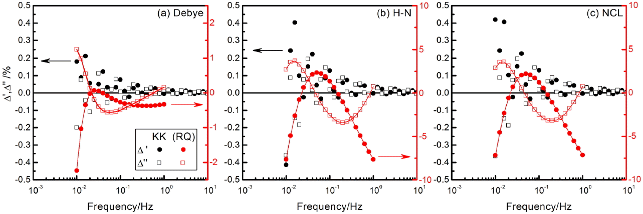
are about 2% for the response generated by Debye relaxations but increase to become as large as 7% for the dispersive responses. The residual errors of the real and imaginary values are shown to be correlated, which suggests the inappropriateness of the modeling. Fig. 6 also presents the residual errors given by the numerical Kramers-Kronig test.8,9) The tests instruct the best possible fit results for the ‘given’ data set and allow a decision to be made as to whether the model can or should be further improved or not. It should be noted however that the numerical KK test program is based on the circuit analysis algorithm using the R, C, L, and Q elements. The algorithm does not work perfectly for the simulated response in the present work, resulting in residual errors as large as 0.4% at the low frequency limit. Similar observations have been made for the simulated data with oscillatory response.39) Residual errors for the same data change with the test frequency range. Simulated data are almost perfectly fitted when the frequency range is chosen appropriately.

One criticism of the impedance analysis is the physical significance of the parameters of the equivalent circuit models when the ‘Maxwell’ and ‘Voigt’ circuits are shown to be exactly equivalent by Eqs. (5) and (6). More significance should be given to the original ‘Maxwell’ circuits in Fig. 2(a) and (b), because the circuit parameters are directly indicated in the raw data presented in Fig. 3. It is notable that C_B in the bricklayer ‘Voigt’ model is higher than the high frequency limit capacitance C_∞= C₀ + C₁. C_B approaches C_∞ = C₀ + C₁ only when C₂ >> C₁. The dielectric constant conventionally estimated from C_B is thus subject to error in this respect in addition to the problem that the true high frequency limit capacitance for the dielectric constant is C₀, not C₀ + C₁.

In the brick-layer model, C_GB is related to the grain boundary layer phase. Space charge theory can explain the presence of continuous grain boundary layers. C_GB/C_B is related to the ratio of the Schottky depletion width to the grain size. The ratio in the present case is 8.55. Space charge layers thus constitute a considerable portion of the grains. This may be considered to be the situation in nanocrystalline solid electrolytes and geometry consideration may be made in the derivation of specific properties from the circuit parameters R_B,GB and C_B,GB.40) In contrast to such conventional approach this work suggests a different description and mechanism for the grain boundary effects.

Impedance spectra in the middle and right columns of Fig. 4(b), (c), and (d) are results from the Havriliak-Negami relaxations obtained using the same time constants as used for the Debye relaxations in the left column. Such spectral feature is indeed experimentally observed. The skewed arcs in the impedance plane are often separated into two (RQ) responses according to the brick-layer model of Fig. 2(c). When the analysis is limited to the data in the visible range, two (RQ) responses would describe the trajectory more or less satisfactorily. As discussed for the data at 1000/T=1, shown in Fig. 4(a), the two resistance components R_B and R_GB are quite different from those in the Debye case. The proportion of the R_B component becomes even less with decreasing temperature. Two conductivity curves from the two components plotted are noted as ‘H-N’ in Fig. 5(a). While the conductivity of R_GB is similar to that of R_T, which has an activation energy of 0.502(± 0.001) eV, R_B corresponds to a distinctly higher conductivity, with a somewhat smaller activation energy of 0.469(± 0.003) eV. The estimated activation energy values for the respective cases are presented in Table 3. The difference in activation energy in this analysis may be regarded as support for the space charge origin of the grain boundary impedance. However, such temperature dependence is not involved in the original simulated data. AC conductivity plots in Fig. 3(g,h,i) indicate the trajectories with activation energy E_σ, no matter whether the response is dispersive or not.

Table 3

Activation Energies Evaluated from the Fit Results by the Brick-Layer Model In Fig. 5(a).

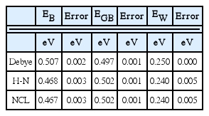
Figure 5(b) indicates that the Q parameters vary arbitrarily, without clear trends. The a values are shown to vary as 0.83, 0.86, and 0.91 for a_B and as 0.90, 0.89, and 0.88 for a_GB. The prefactors are shown to decrease with temperature. The six parameters for the brick-layer models adjust to each other to yield the least sum of squares. They are closely correlated with each other and thus do not provide trends of physical significance. The sum of squares or the χ² values become larger by orders of magnitude compared to the Debye case, as shown in Table 2.

While the ratio C_GB/C_B is 8.55 in the Debye case, the capacitance effects, represented by the prefactors of Q, are shown to be higher in Q_B than in Q_GB. The relaxation time constants τ = (RQ)^1/a are largely determined by the resistance values with R_GB >> R_B. The effective capacitance ‘C’ from the depressed semicircular response is conventionally estimated as ‘C ’ = τR⁻¹ = (RQ)^1/aR⁻¹.40–45) The estimates are also presented in Fig. 5(b). For the response with Debye relaxations with a close to one, ‘C ’ and Q almost coincide with each other. The difference between the Q factors for the dispersive responses is reduced but ‘C_B’ is still higher than ‘C_GB’. The results cannot be explained by the brick layer model. ‘C_GB’ becomes larger than ‘C_B’ when R_GB is much larger than R_B and/or when C₂/C₁ is larger than in the present example. Fundamental physical significance would be difficult to be provided for these parameters.

In Fig. 5, for the results of the brick-layer analysis, only the results of the data for the Debye and H-N relaxations are presented. There are small differences due to the dielectric loss factor with a₀=0.995, as shown in Table 2, but these differences are hardly distinguishable in the logarithmic plots. The upper frequency range is cut off, so that the high frequency limit capacitance becomes C_∞ = C₀ + C₁. Therefore, the effects of the dielectric loss associated with the C₀ element are modest. As noted above, the high frequency capacitance C_∞ = C₀ + C₁ does not, however, represent a true dielectric constant. As illustrated in the series of capacitance Bode plots shown in Fig. 3(a,b,c), true geometric capacitance C₀ at high frequency limit can be directly measured at sufficiently low temperature for solid electrolyte systems, which are characterized by small R_T or R_B, large C₁, and small τ₁ (or a high response frequency range).

When the fitting range includes the squashed high frequency region, which is very likely in the practice, the relaxation from C₀ to C₀+C₁ should be appropriately modeled. Parallel (RQC₀) models as indicated in the equivalent circuit in Fig. 2(c) have been shown to describe experimental spectra satisfactorily,46–50) although no definite characterization or understanding of the dispersive behavior has been made. The frequency dispersion due to the mobile charge carriers, characterized by ‘H₁,’ a Cole-Davidson response with γ≈0.4, can be approximated by Q with a≈0.6 on the high frequency side. High frequency dispersion of solid electrolytes is thus more appropriately approximated by Q in parallel to C₀.51) Dielectric loss can also be represented by a slight non-ideality in C₀.

Conductivity (real admittance) spectra have generally been preferred to indicate the frequency dispersion, because almost ideal geometric capacitance does not contribute to real admittance. In the description of the spectra both in real and imaginary quantities, the presence of parallel capacitance C₀ is essential. Well-defined capacitance magnitudes and frequency dispersion can be described by the complex dielectric functions in Eq. (1) and by the modeling in Fig. 2(b). It should be mentioned that such behavior is not limited to current-constriction type solid electrolytes but to the systems that exhibit grain boundary effects with temperature dependence clearly distinct from that of the bulk. Proton conducting barium zirconates with huge grain boundary effects can be included in this category. The space charge analysis described above has so far been applied.43–45) These systems exhibit rather involved grain boundary effects, apparently with multiple relaxations. The present method can be extended to tackle such nontrivial behavior and to find the correct physics behind it.

For the spectra in Fig. 4(a) and (b) at 1000/T = 1 and 2, the parameters of the Warburg response are fitted close to the original values in Fig. 2(a,b). This holds for the spectrum on the left in Fig. 4(c) at 1000/T = 3, generated by Debye relaxations. The sample response described by the almost ideal nondispersive capacitance elements does not overlap significantly with the low frequency range response. The Warburg response in the fitting range is sufficient to yield close-to-original parameters. This is not true for the dispersive responses generated by Havriliak-Negami relaxations, however. When the dispersive responses are approximately described by Q elements with a significantly less than 1, e.g. 0.9, the CPE response extends over a wide frequency range. The observed Warburg response should thus be described together with Q element(s) in the brick-layer model. This results in a value of a_W=0.57, significantly different from the original ideal value of 0.5, as can be seen in Fig. 5(a) and in Table 2. The original Warburg parameters were obtained for the dispersive spectra at higher temperature at 1000/T = 1 and 2 shown in Fig. 4(a) and (b) due to the wide coverage of the Warburg response in the analysis frequency range. The correlated deviation in the Q_W values is indicated in the activation energy of Q_W, estimated to be 0.240(±0.005) eV, in comparison with the value of 0.250 eV for the Debye case (Table 3). This again illustrates the caution against the unjustified employment of ‘magic’ Q elements.

5. Conclusions

Brick-layer modeling with constant phase elements as generalized capacitance elements for polycrystalline solid electrolytes cannot satisfactorily describe the experimental spectra over a wide range and the physical significance of the parameters derived there from is rather weak. Strongly dispersive responses in fact indicate well-defined capacitance values and frequency dependence. Modeling based on such observations allows a description of the AC response over a wide temperature and frequency range with a very limited number of parameters—around ten. A comprehensive and definite electrical characterization of the solid electrolyte materials and their devices can be finally made.

Article information Continued